Ten-Minute Tutorial

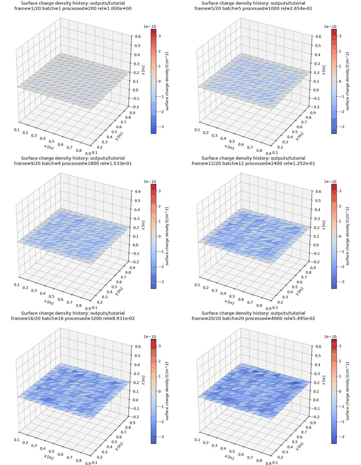
This tutorial injects 200 macro-electrons per batch, 4,000 in total, toward an insulating plane for 20 batches. It shows a surface-charge distribution forming at absorption locations and the accumulated field beginning to reflect electrons in later batches.

The case is designed to expose BEACH’s batch-to-batch feedback. It is not a calibrated research environment and does not claim a steady state or convergence in physical time.

0. Check the installation

beach --version
beachx --help

If both commands run, continue. Otherwise, see Installation. On an HPC login node, do not run the simulation directly; execute the remaining commands inside a compute-node allocation.

1. Create the configuration

mkdir beach-tutorial
cd beach-tutorial
beachx config init beach.toml
beachx lint beach.toml

The generated settings and behavior are identical to examples/tutorial_insulator.toml. Comments, array wrapping, and other TOML formatting may differ. You do not need to memorize the full file. Start with these relationships.

Setting	Value	Role in this case
sim.batch_count	20	Repeat charge commit and field refresh 20 times
sim.dt / sim.max_step	5e-8 s / 80	Integrate each electron trajectory
sim.field_solver / field_boundary.mode	direct / free	Evaluate the finite plane’s free-space field with Direct BEM
npcls_per_step	200	Create 200 macro-electrons in every batch
w_particle	2e5	Represent 200,000 electrons with each macro-electron so feedback appears in a short run
pos_low / pos_high	rectangle at z = 0.8 m	Sample injection positions across a broad region above the plane
drift_velocity	[0, 0, -1e6] m/s	Direct electrons toward the plane
mesh.templates	12 × 12 cells	Divide the plane into 288 triangles
history_stride / write_potential_history	1 / true	Save charge and potential after every batch

Every particle in one batch uses the same field fixed at the start of that batch. Absorbed charge is committed once at the batch end and changes the field first used by the next batch. This sequence is central to BEACH.

2. Run the case

Use one OpenMP thread here to reproduce the reference random sequence.

OMP_NUM_THREADS=1 beach beach.toml
beachx inspect outputs/tutorial

A successful reference run reports:

processed_particles=4000
absorbed=3720 escaped=280
batches=20
charge_sum=-1.192019e-10
potential_min=-4.671330e+00
potential_max=-2.579807e+00

processed_particles=200 × 20 and batches=20 follow exactly from the configuration. The absorption, escape, and potential values above are references for rng_seed=12345, one thread, and the current version. Fine details may change with another thread count or a future random-number implementation.

3. Why electrons escape in later batches

All 200 electrons are absorbed in each of the first 13 batches. As negative charge accumulates, the surface potential becomes more negative and produces a field that opposes incoming electrons. Starting in batch 14, some electrons turn around and leave through the upper open boundary.

The final surface charge is

$$3720\times 2\times10^5\times(-e) =-1.192019\times10^{-10}\ \mathrm{C},$$

which agrees with charge_sum. The charge_C column in charges.csv is total charge [C] on each triangle. Plot colors show that charge divided by triangle area, in C/m².

For this finite free-space surface, the Coulomb-potential convention approaches 0 V in the far field. No matching plane or reservoir.phi_infty is connected, so do not reinterpret this potential as an outer-plasma potential.

4. View charge history and final potential

beachx inspect outputs/tutorial \
  --save-mesh outputs/tutorial/charge.png

beachx animate outputs/tutorial \
  --quantity charge \
  --save-gif outputs/tutorial/charge_history.gif \
  --total-frames 20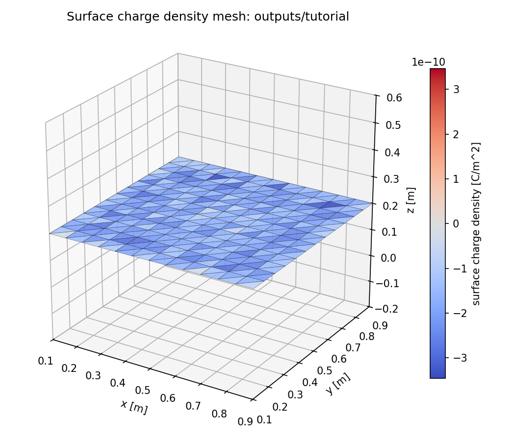

The final surface potential is already stored in mesh_potential.csv. Plot the saved values without recomputation by setting reference_point=None explicitly.

from beach import Beach

run = Beach("outputs/tutorial", config_path="beach.toml")
fig, _ = run.plot_potential(reference_point=None)
fig.savefig("outputs/tutorial/potential.png", dpi=150)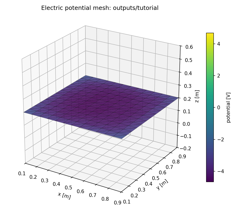

Reconstructing potential at arbitrary points or for every batch requires the native field kernel. Follow the optional steps in the Post-processing Tutorial when you need that calculation.

5. What this result does and does not show

This run demonstrates that particle generation, orbit integration, collision and escape, element-wise charge commit, field refresh, and history output are coupled across batches.

However, w_particle is a teaching value selected to expose feedback quickly, and a volume_seed with batch_duration=0 has no physical inflow rate in seconds. last_rel_change and tol_rel are not automatic stopping conditions. Do not interpret these 20 batches as a steady charging state or as 20 seconds in a particular environment.

6. Continue

Goal	Next page
Check output files and conservation	Inspect output files
Resume once from the 20-batch checkpoint	Run and resume
Change particle counts, geometry, or sources	Design a simulation case
Understand batches, particles, and charge commits	What BEACH solves and how a run advances
Decide whether a research result is acceptable	Validating simulation results
Diagnose a failed run	Troubleshooting